Editor

How to Use Pandas Online: No Installation Required

Beginner15 min0 exercises0 XP

You want to load a CSV, filter some rows, group by category, and plot the result. The standard path: install Python, create a virtual environment, run pip install pandas matplotlib, open Jupyter. Twenty minutes later you're still fixing a conda conflict.

The shortcut: open pythoncompiler.io in a browser tab. Pandas, NumPy, and Matplotlib load the first time you import them. No installation, no account, no waiting. Your first analysis can be running in under 60 seconds.

This guide walks through the most useful Pandas operations - all with runnable examples you can edit and execute directly on this page.

Create and Explore a DataFrame

A Pandas DataFrame is a table with named columns and a row index. You can build one from a dictionary, a list of dicts, a CSV, or many other sources.

Create and inspect a DataFrame
import pandas as pd
# Build a DataFrame from a dictionary
sales = pd.DataFrame({
'month': ['Jan', 'Feb', 'Mar', 'Apr', 'May', 'Jun'],
'region': ['North', 'South', 'North', 'South', 'North', 'South'],
'revenue': [12400, 9800, 15600, 11200, 18900, 14300],
'units': [124, 98, 156, 112, 189, 143],
})
print(sales)
print()
print("Shape:", sales.shape)
print("Columns:", list(sales.columns))
print()
print(sales.describe())
Output
  month region  revenue  units
0   Jan  North    12400    124
1   Feb  South     9800     98
2   Mar  North    15600    156
3   Apr  South    11200    112
4   May  North    18900    189
5   Jun  South    14300    143

Shape: (6, 4)
Columns: ['month', 'region', 'revenue', 'units']

            revenue       units
count      6.000000    6.000000
mean   13700.000000  137.000000
std     3291.200389   32.912004
min     9800.000000   98.000000
25%    11500.000000  115.000000
50%    13350.000000  133.500000
75%    15275.000000  152.750000
max    18900.000000  189.000000

Load Data from a CSV

In a real project you'd use pd.read_csv("file.csv"). In the browser, use io.StringIO to wrap an inline CSV string - the same API, perfect for testing and learning.

Load CSV data inline
import pandas as pd
import io
csv_data = """product,category,price,stock
Laptop,Electronics,999,45
Headphones,Electronics,79,312
Desk,Furniture,349,28
Chair,Furniture,189,74
Notebook,Stationery,5,890
Pen,Stationery,2,2100"""
df = pd.read_csv(io.StringIO(csv_data))
print(df)
print()
print("Data types:")
print(df.dtypes)
Output
      product     category  price  stock
0      Laptop  Electronics    999     45
1  Headphones  Electronics     79    312
2        Desk    Furniture    349     28
3       Chair    Furniture    189     74
4    Notebook   Stationery      5    890
5         Pen   Stationery      2   2100

Data types:
product     object
category    object
price        int64
stock        int64
dtype: object

Filter, Sort, and Select

Boolean indexing is the core of Pandas filtering. Pass any True/False condition inside df[...] to select matching rows.

Filter and sort data
import pandas as pd
import io
csv_data = """product,category,price,stock
Laptop,Electronics,999,45
Headphones,Electronics,79,312
Desk,Furniture,349,28
Chair,Furniture,189,74
Notebook,Stationery,5,890
Pen,Stationery,2,2100"""
df = pd.read_csv(io.StringIO(csv_data))
# Filter: price > 100
expensive = df[df['price'] > 100]
print("Items over $100:")
print(expensive[['product', 'price']])
print()
# Multiple conditions
electronics_cheap = df[(df['category'] == 'Electronics') & (df['price'] < 200)]
print("Affordable electronics:")
print(electronics_cheap)
print()
# Sort by price descending
print("By price (high to low):")
print(df.sort_values('price', ascending=False)[['product', 'price']].head(3))
Output
Items over $100:
  product  price
0  Laptop    999
2    Desk    349
3   Chair    189

Affordable electronics:
      product     category  price  stock
1  Headphones  Electronics     79    312

By price (high to low):
  product  price
0  Laptop    999
2    Desk    349
3   Chair    189

GroupBy and Aggregate

groupby splits your DataFrame into groups, lets you apply a function to each, and combines the results. This is the Pandas equivalent of SQL's GROUP BY - and it's one of the most powerful tools in data analysis.

GroupBy with multiple aggregations
import pandas as pd
sales = pd.DataFrame({
'month': ['Jan','Feb','Mar','Apr','May','Jun','Jan','Feb','Mar'],
'region': ['North','North','North','South','South','South','West','West','West'],
'revenue': [12400, 9800, 15600, 11200, 18900, 14300, 8700, 11400, 9200],
'units': [124, 98, 156, 112, 189, 143, 87, 114, 92],
})
# Total revenue per region
by_region = sales.groupby('region')['revenue'].sum().sort_values(ascending=False)
print("Revenue by region:")
print(by_region)
print()
# Multiple aggregations
summary = sales.groupby('region').agg(
total_revenue=('revenue', 'sum'),
avg_revenue=('revenue', 'mean'),
total_units=('units', 'sum'),
months=('month', 'count'),
).round(0)
print("Full summary:")
print(summary)
Output
Revenue by region:
region
South    44400
North    37800
West     29300
Name: revenue, dtype: int64

Full summary:
        total_revenue  avg_revenue  total_units  months
region                                                 
North           37800      12600.0          378       3
South           44400      14800.0          444       3
West            29300       9767.0          293       3

Merge Two DataFrames

Pandas merge works like a SQL JOIN - combine two DataFrames on a shared key. Supports inner, left, right, and outer joins.

Merge orders with customer data
import pandas as pd
orders = pd.DataFrame({
'order_id': [1, 2, 3, 4, 5],
'customer_id': [101, 102, 101, 103, 102],
'amount': [250, 80, 175, 320, 95],
})
customers = pd.DataFrame({
'customer_id': [101, 102, 103],
'name': ['Alice', 'Bob', 'Charlie'],
'tier': ['Gold', 'Silver', 'Gold'],
})
# Inner join on customer_id
merged = pd.merge(orders, customers, on='customer_id')
print(merged)
print()
# Total spend per customer
total = merged.groupby('name')['amount'].sum().sort_values(ascending=False)
print("Total spend per customer:")
print(total)
Output
   order_id  customer_id  amount     name    tier
0         1          101     250    Alice    Gold
1         2          102      80      Bob  Silver
2         3          101     175    Alice    Gold
3         4          103     320  Charlie    Gold
4         5          102      95      Bob  Silver

Total spend per customer:
name
Alice      425
Charlie    320
Bob        175
Name: amount, dtype: int64

Visualize with Matplotlib

Pandas integrates directly with Matplotlib. Call .plot() on any Series or DataFrame column to create a chart. The plot renders in the output panel below your code.
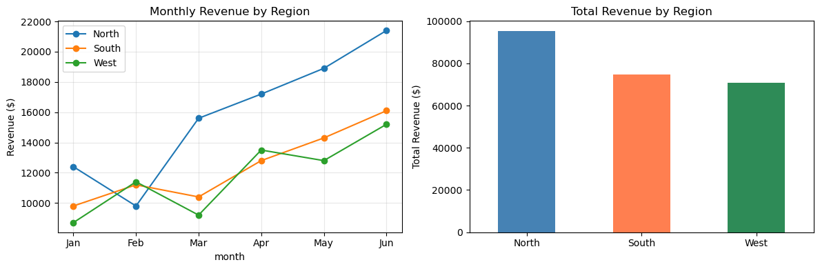
Multi-chart Pandas visualization
import pandas as pd
import matplotlib.pyplot as plt
sales = pd.DataFrame({
'month': ['Jan','Feb','Mar','Apr','May','Jun'],
'North': [12400, 9800, 15600, 17200, 18900, 21400],
'South': [9800, 11200, 10400, 12800, 14300, 16100],
'West': [8700, 11400, 9200, 13500, 12800, 15200],
}).set_index('month')
fig, axes = plt.subplots(1, 2, figsize=(12, 4))
# Line chart: revenue over time by region
sales.plot(ax=axes[0], marker='o', title='Monthly Revenue by Region')
axes[0].set_ylabel('Revenue ($)')
axes[0].grid(True, alpha=0.3)
# Bar chart: total by region
sales.sum().plot(kind='bar', ax=axes[1], color=['steelblue','coral','seagreen'],
title='Total Revenue by Region', rot=0)
axes[1].set_ylabel('Total Revenue ($)')
plt.tight_layout()
plt.show()
Output
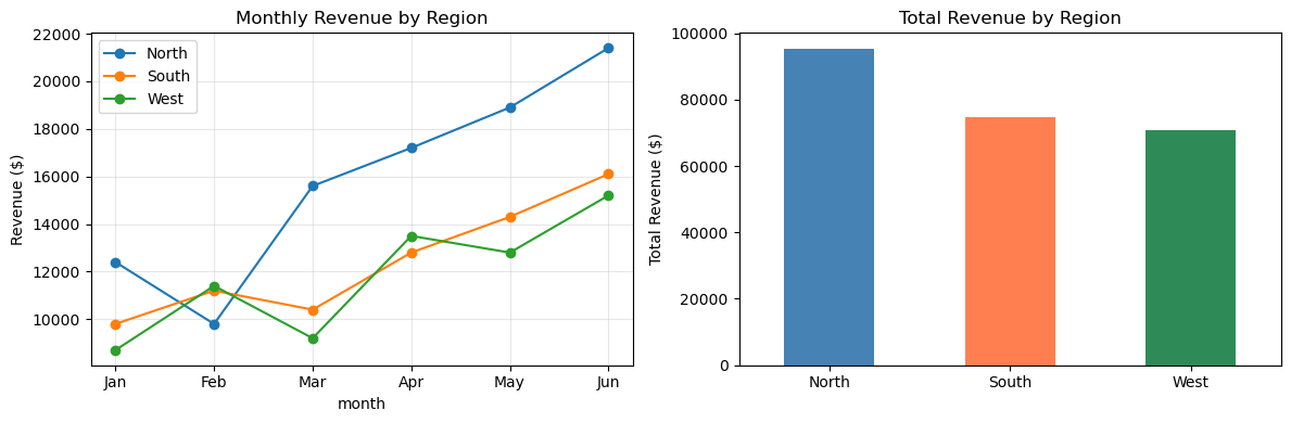
Chart drawn by: Multi-chart Pandas visualizationChart drawn by: Multi-chart Pandas visualization

Install Additional Packages

Pandas, NumPy, and Matplotlib load automatically. For more libraries - scikit-learn, scipy, statsmodels, seaborn - open the Packages panel on the right side of the editor and install them on demand. Everything runs locally in your browser - no server, no rate limits.

Linear regression with scikit-learn (install from Packages panel)
# After installing scikit-learn from the Packages panel:
import pandas as pd
import numpy as np
from sklearn.linear_model import LinearRegression
# Simulate housing data
np.random.seed(42)
n = 100
df = pd.DataFrame({
'sqft': np.random.randint(500, 3000, n),
'beds': np.random.randint(1, 6, n),
'price': np.random.randint(100000, 800000, n),
})
df['price'] = df['sqft'] * 200 + df['beds'] * 15000 + np.random.randn(n) * 20000
X = df[['sqft', 'beds']]
y = df['price']
model = LinearRegression().fit(X, y)
print(f"R² score: {model.score(X, y):.3f}")
print(f"Price per sqft: ${model.coef_[0]:,.0f}")
print(f"Price per bedroom: ${model.coef_[1]:,.0f}")
print(f"Predicted price (1200sqft, 3 beds): ${model.predict([[1200, 3]])[0]:,.0f}")
Output
R² score: 0.979
Price per sqft: $201
Price per bedroom: $15,751
Predicted price (1200sqft, 3 beds): $283,690
/lib/python3.13/site-packages/sklearn/utils/validation.py:2749: UserWarning: X does not have valid feature names, but LinearRegression was fitted with feature names
  warnings.warn(

Harder problems

More problems on this topic: Working with data

Related Tutorials

Was this tutorial helpful?