Editor

Matplotlib: Create Line, Bar, Scatter, and Pie Charts

Intermediate25 min6 exercises90 XP
0/6 exercises

Imagine you have a spreadsheet with 10,000 rows of sales data. You could stare at those numbers for hours, or you could turn them into a chart and spot the trend in three seconds. That's the power of data visualization.

Matplotlib is Python's most popular plotting library. It's been around since 2003, and virtually every data science chart you've seen in Python was made with it (or a library built on top of it). In this tutorial, you'll learn how to create line charts, bar charts, scatter plots, and more.

How Do You Create a Basic Line Chart?

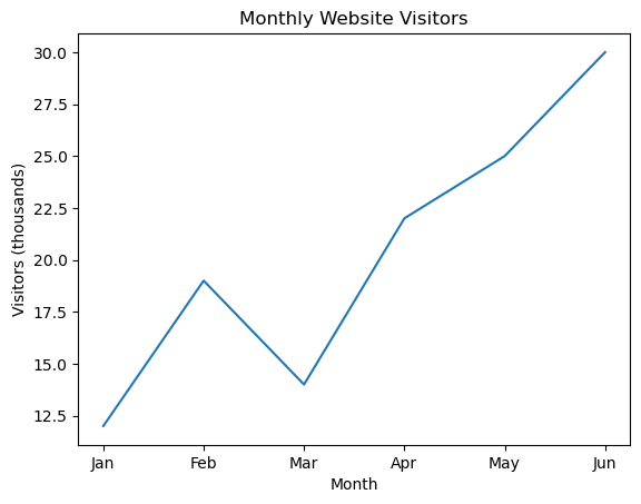
A line chart connects data points with straight lines. It's perfect for showing how something changes over time - stock prices, temperatures, website visitors.

In matplotlib, you give it two lists: one for the x-axis (horizontal) and one for the y-axis (vertical). Each pair of values becomes a point, and matplotlib draws lines between them.

Creating a basic line chart
import matplotlib
matplotlib.use('Agg') # Non-interactive backend
import matplotlib.pyplot as plt
# Monthly website visitors (in thousands)
months = ['Jan', 'Feb', 'Mar', 'Apr', 'May', 'Jun']
visitors = [12, 19, 14, 22, 25, 30]
# Create the plot
fig, ax = plt.subplots()
ax.plot(months, visitors)
ax.set_title('Monthly Website Visitors')
ax.set_xlabel('Month')
ax.set_ylabel('Visitors (thousands)')
# Verify our chart configuration
print('Title:', ax.get_title())
print('X label:', ax.get_xlabel())
print('Y label:', ax.get_ylabel())
print('Number of lines:', len(ax.lines))
print('Data points:', len(ax.lines[0].get_xdata()))
Output
Title: Monthly Website Visitors
X label: Month
Y label: Visitors (thousands)
Number of lines: 1
Data points: 6
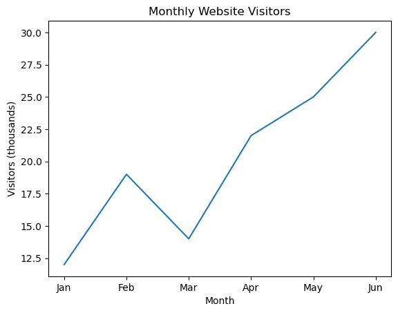
Chart drawn by: Creating a basic line chartChart drawn by: Creating a basic line chart

Notice we used fig, ax = plt.subplots(). This is the recommended way to create plots in matplotlib. fig is the whole figure (like a canvas), and ax is the axes (the actual chart area where data gets drawn).

When Should You Use a Bar Chart?

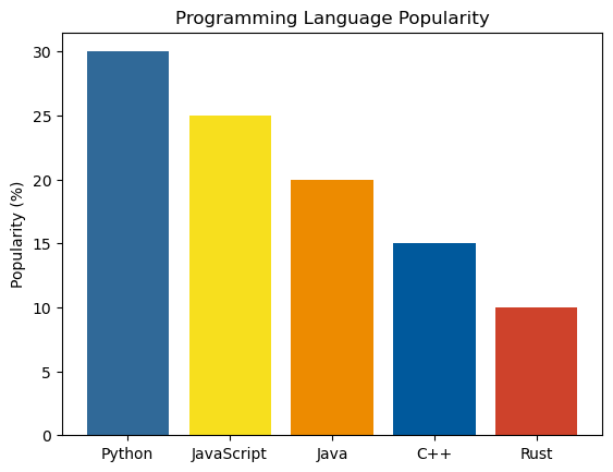
Bar charts are ideal for comparing categories. How did each product sell? Which city has the most population? Whenever you're comparing distinct groups, a bar chart is your best bet.

Creating a bar chart with custom colors
import matplotlib
matplotlib.use('Agg')
import matplotlib.pyplot as plt
# Programming language popularity
languages = ['Python', 'JavaScript', 'Java', 'C++', 'Rust']
popularity = [30, 25, 20, 15, 10]
fig, ax = plt.subplots()
bars = ax.bar(languages, popularity, color=['#306998', '#F7DF1E', '#ED8B00', '#00599C', '#CE422B'])
ax.set_title('Programming Language Popularity')
ax.set_ylabel('Popularity (%)')
# Verify the chart
print('Number of bars:', len(bars))
print('Bar heights:', [b.get_height() for b in bars])
print('Title:', ax.get_title())
Output
Number of bars: 5
Bar heights: [np.int32(30), np.int32(25), np.int32(20), np.int32(15), np.int32(10)]
Title: Programming Language Popularity
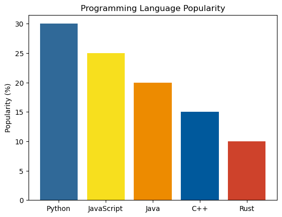
Chart drawn by: Creating a bar chart with custom colorsChart drawn by: Creating a bar chart with custom colors

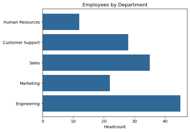
You can also create horizontal bar charts using ax.barh(). These work great when your category labels are long - they're easier to read horizontally.

Horizontal bar chart
import matplotlib
matplotlib.use('Agg')
import matplotlib.pyplot as plt
# Employee departments
departments = ['Engineering', 'Marketing', 'Sales', 'Customer Support', 'Human Resources']
headcount = [45, 22, 35, 28, 12]
fig, ax = plt.subplots()
ax.barh(departments, headcount, color='#306998')
ax.set_title('Employees by Department')
ax.set_xlabel('Headcount')
print('Chart type: horizontal bar')
print('Departments:', len(departments))
print('Largest department:', departments[headcount.index(max(headcount))], 'with', max(headcount), 'employees')
Output
Chart type: horizontal bar
Departments: 5
Largest department: Engineering with 45 employees
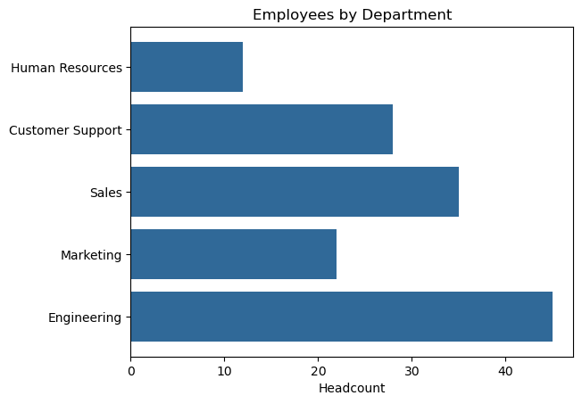
Chart drawn by: Horizontal bar chartChart drawn by: Horizontal bar chart

How Do Scatter Plots Reveal Relationships?

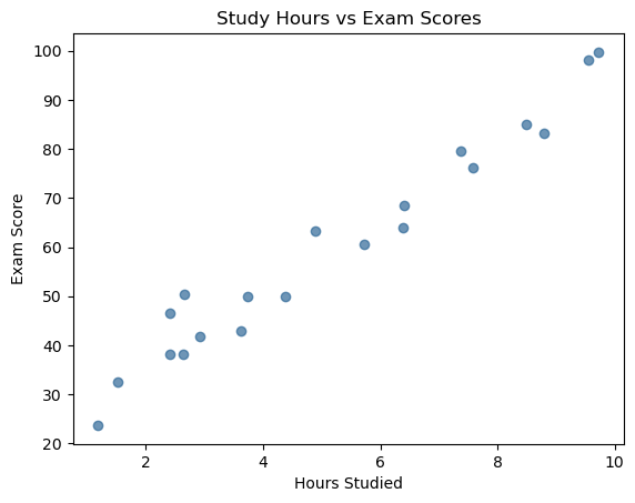
Scatter plots show how two variables relate to each other. Each dot represents one data point, positioned by its x and y values. If the dots trend upward, there's a positive correlation. If they trend downward, it's negative. If they're scattered randomly, there's no clear relationship.

Think of a scatter plot like a map. Each dot is a person, and their position tells you two things about them simultaneously - like hours studied vs. exam score.

Scatter plot showing correlation
import matplotlib
matplotlib.use('Agg')
import matplotlib.pyplot as plt
import numpy as np
# Study hours vs exam scores
np.random.seed(42)
hours_studied = np.random.uniform(1, 10, 20)
exam_scores = hours_studied * 8 + np.random.normal(0, 5, 20) + 20
fig, ax = plt.subplots()
ax.scatter(hours_studied, exam_scores, color='#306998', alpha=0.7)
ax.set_title('Study Hours vs Exam Scores')
ax.set_xlabel('Hours Studied')
ax.set_ylabel('Exam Score')
print('Number of data points:', len(hours_studied))
print('Hours range: {:.1f} to {:.1f}'.format(min(hours_studied), max(hours_studied)))
print('Score range: {:.1f} to {:.1f}'.format(min(exam_scores), max(exam_scores)))
# Check correlation
correlation = np.corrcoef(hours_studied, exam_scores)[0, 1]
print(f'Correlation: {correlation:.2f} (strong positive)')
Output
Number of data points: 20
Hours range: 1.2 to 9.7
Score range: 23.7 to 99.7
Correlation: 0.98 (strong positive)
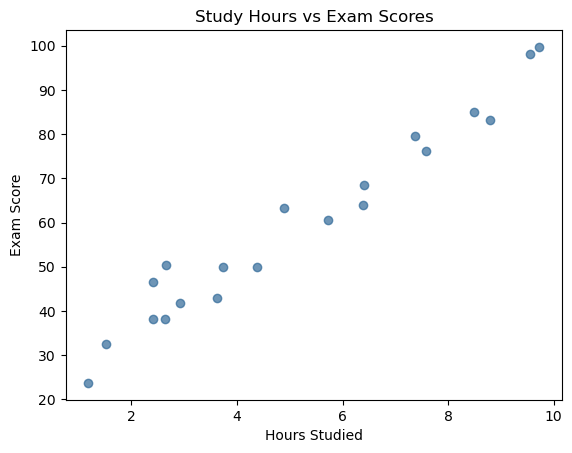
Chart drawn by: Scatter plot showing correlationChart drawn by: Scatter plot showing correlation

How Do You Customize Colors, Markers, and Styles?

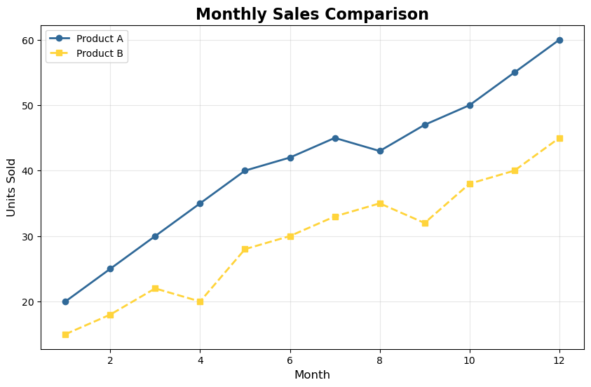
A chart without customization is like a report without formatting - it works, but nobody wants to read it. Matplotlib gives you full control over colors, line styles, markers, and fonts.

Customized line chart with legend and grid
import matplotlib
matplotlib.use('Agg')
import matplotlib.pyplot as plt
months = list(range(1, 13))
product_a = [20, 25, 30, 35, 40, 42, 45, 43, 47, 50, 55, 60]
product_b = [15, 18, 22, 20, 28, 30, 33, 35, 32, 38, 40, 45]
fig, ax = plt.subplots(figsize=(10, 6))
# Line with markers and custom style
ax.plot(months, product_a, color='#306998', linewidth=2,
marker='o', markersize=6, label='Product A')
ax.plot(months, product_b, color='#FFD43B', linewidth=2,
linestyle='--', marker='s', markersize=6, label='Product B')
ax.set_title('Monthly Sales Comparison', fontsize=16, fontweight='bold')
ax.set_xlabel('Month', fontsize=12)
ax.set_ylabel('Units Sold', fontsize=12)
ax.legend()
ax.grid(True, alpha=0.3)
print('Figure size:', fig.get_size_inches())
print('Number of lines:', len(ax.lines))
print('Legend entries:', [t.get_text() for t in ax.get_legend().get_texts()])
print('Grid visible:', ax.xaxis.get_gridlines()[0].get_visible())
Output
Figure size: [10.  6.]
Number of lines: 2
Legend entries: ['Product A', 'Product B']
Grid visible: True
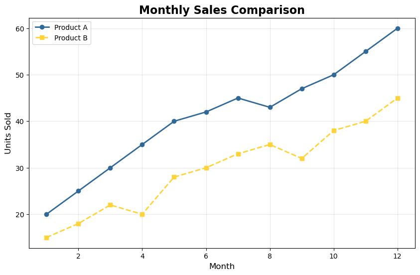
Chart drawn by: Customized line chart with legend and gridChart drawn by: Customized line chart with legend and grid

Here's a quick reference for common line styles and markers:

Quick reference for styles and markers
# Line styles
# '-' solid line (default)
# '--' dashed line
# '-.' dash-dot line
# ':' dotted line
# Common markers
# 'o' circle
# 's' square
# '^' triangle up
# 'D' diamond
# '*' star
# '+' plus
# 'x' cross
print('Line styles: solid(-), dashed(--), dash-dot(-.), dotted(:)')
print('Markers: o, s, ^, D, *, +, x')
Output
Line styles: solid(-), dashed(--), dash-dot(-.), dotted(:)
Markers: o, s, ^, D, *, +, x

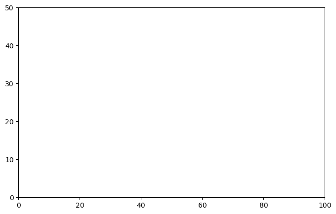
What's the Difference Between Figure and Axes?

Understanding the relationship between Figure and Axes is the key to mastering matplotlib. Think of it like a picture frame and a photo:

  • Figure = the entire window or image. It's the frame that holds everything.
  • Axes = one individual chart inside the figure. A figure can contain multiple axes.
  • Axis = one side of the chart (x-axis, y-axis). Each axes object has two axis objects.
  • Figure vs axes
    import matplotlib
    matplotlib.use('Agg')
    import matplotlib.pyplot as plt
    # Create a figure with specific size
    fig, ax = plt.subplots(figsize=(8, 5))
    # The figure controls the canvas
    print('Figure size (inches):', fig.get_size_inches())
    print('Figure DPI:', fig.dpi)
    print('Figure dimensions in pixels: {:.0f} x {:.0f}'.format(
    fig.get_size_inches()[0] * fig.dpi,
    fig.get_size_inches()[1] * fig.dpi
    ))
    # The axes controls the chart content
    ax.set_xlim(0, 100)
    ax.set_ylim(0, 50)
    print('X limits:', ax.get_xlim())
    print('Y limits:', ax.get_ylim())
    Output
    Figure size (inches): [8. 5.]
    Figure DPI: 100.0
    Figure dimensions in pixels: 800 x 500
    X limits: (np.float64(0.0), np.float64(100.0))
    Y limits: (np.float64(0.0), np.float64(50.0))
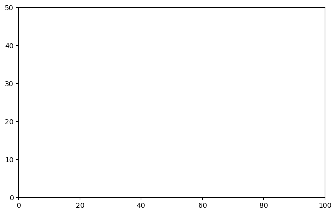
    Chart drawn by: Figure vs axesChart drawn by: Figure vs axes

    How Do You Save Charts to Files?

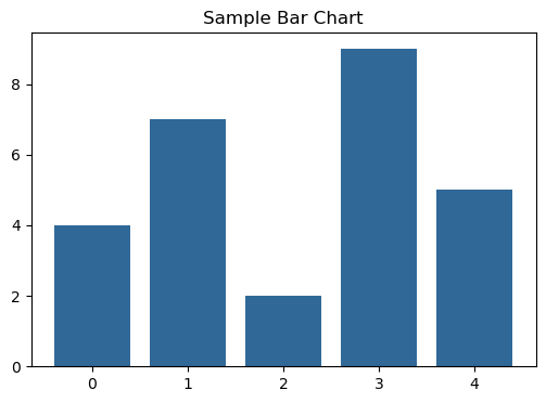
    In a real project, you'll want to save your charts as image files to include in reports, presentations, or web pages. Matplotlib supports PNG, PDF, SVG, and more.

    Saving charts to files
    import matplotlib
    matplotlib.use('Agg')
    import matplotlib.pyplot as plt
    data = [4, 7, 2, 9, 5]
    fig, ax = plt.subplots(figsize=(6, 4))
    ax.bar(range(len(data)), data, color='#306998')
    ax.set_title('Sample Bar Chart')
    # Save to different formats
    # fig.savefig('chart.png', dpi=150, bbox_inches='tight')
    # fig.savefig('chart.pdf', bbox_inches='tight')
    # fig.savefig('chart.svg', bbox_inches='tight')
    # We can't save files here, but let's verify the setup
    print('Supported formats:', list(fig.canvas.get_supported_filetypes().keys())[:6])
    print('DPI:', fig.dpi)
    print('Figure size:', fig.get_size_inches())
    print('bbox_inches="tight" removes extra whitespace around the chart')
    Output
    Supported formats: ['eps', 'jpg', 'jpeg', 'pdf', 'pgf', 'png']
    DPI: 100.0
    Figure size: [6. 4.]
    bbox_inches="tight" removes extra whitespace around the chart
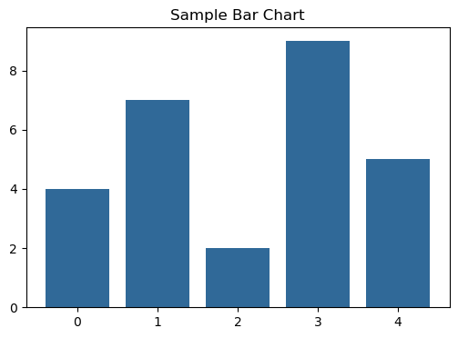
    Chart drawn by: Saving charts to filesChart drawn by: Saving charts to files

    Practice Exercises

    Build a Temperature Line Chart
    Write Code

    Create a line chart showing daily temperatures. Use matplotlib.use('Agg') first, then create a figure with plt.subplots(). Plot the temperatures list against the days list. Set the title to 'Daily Temperatures', the x-label to 'Day', and the y-label to 'Temperature (F)'. Finally, print the title using ax.get_title().

    import matplotlib
    matplotlib.use('Agg')
    import matplotlib.pyplot as plt
    days = ['Mon', 'Tue', 'Wed', 'Thu', 'Fri', 'Sat', 'Sun']
    temperatures = [72, 75, 68, 70, 78, 82, 79]
    # Create figure and axes
    # Plot the data
    # Set title and labels
    # Print the title
    Build a Fruit Sales Bar Chart
    Write Code

    Create a bar chart showing fruit sales. Plot fruits on the x-axis and sales on the y-axis using ax.bar(). Set the title to 'Fruit Sales'. Print the number of bars using len(ax.patches) and print the height of the tallest bar.

    import matplotlib
    matplotlib.use('Agg')
    import matplotlib.pyplot as plt
    fruits = ['Apples', 'Bananas', 'Cherries', 'Dates']
    sales = [150, 200, 80, 120]
    # Create figure, plot bars, set title
    # Print number of bars
    # Print tallest bar height
    Create a Height vs Weight Scatter Plot
    Write Code

    Create a scatter plot of height vs weight data. Use ax.scatter() with alpha=0.6. Set the title to 'Height vs Weight'. Print the number of data points in the scatter collection using len(ax.collections[0].get_offsets()).

    import matplotlib
    matplotlib.use('Agg')
    import matplotlib.pyplot as plt
    heights = [160, 165, 170, 175, 180, 185, 170, 168, 172, 178]
    weights = [55, 62, 68, 74, 80, 85, 65, 60, 70, 76]
    # Create scatter plot with alpha=0.6
    # Set title
    # Print number of data points
    Predict the Figure Properties
    Predict Output

    What will this code print? Think about figure dimensions and line count.

    import matplotlib
    matplotlib.use('Agg')
    import matplotlib.pyplot as plt
    fig, ax = plt.subplots(figsize=(12, 8))
    ax.plot([1, 2, 3], [10, 20, 30], label='A')
    ax.plot([1, 2, 3], [30, 20, 10], label='B')
    ax.set_title('Two Lines')
    print(fig.get_size_inches()[0])
    print(len(ax.lines))
    Fix the Broken Legend
    Fix the Bug

    This code tries to create a chart with a legend, but the legend shows no entries. Fix the bug so the legend displays ['Revenue', 'Expenses'].

    import matplotlib
    matplotlib.use('Agg')
    import matplotlib.pyplot as plt
    months = [1, 2, 3, 4, 5]
    revenue = [100, 120, 140, 160, 180]
    expenses = [90, 95, 100, 110, 115]
    fig, ax = plt.subplots()
    ax.plot(months, revenue)
    ax.plot(months, expenses)
    ax.legend()
    legend_texts = [t.get_text() for t in ax.get_legend().get_texts()]
    print(legend_texts)
    Prepare Data for a Multi-Series Chart
    Write Code

    You have quarterly revenue data for three products. Create a grouped bar chart by computing the x-positions for each group. Given quarters (4 items) and bar width 0.25, calculate x positions for three product groups so bars sit side by side. Print the x positions for each product as lists (use .tolist() to convert numpy arrays). Product A should be at positions [0, 1, 2, 3], Product B at [0.25, 1.25, 2.25, 3.25], and Product C at [0.5, 1.5, 2.5, 3.5].

    import numpy as np
    quarters = ['Q1', 'Q2', 'Q3', 'Q4']
    revenue_a = [50, 60, 70, 80]
    revenue_b = [40, 55, 65, 75]
    revenue_c = [30, 45, 55, 70]
    width = 0.25
    x = np.arange(len(quarters)) # [0, 1, 2, 3]
    # Calculate positions for each product group
    pos_a = x # First group at base positions
    # Calculate pos_b and pos_c
    print(pos_a.tolist())
    # Print pos_b and pos_c as lists

    Harder problems

    More problems on this topic: Working with data

    Related Tutorials

    Was this tutorial helpful?