Editor

Advanced Matplotlib: Subplots, Dual Axes, Styles, Annotations

Advanced25 min5 exercises100 XP
0/5 exercises

You know how to create a single chart. But real-world reports rarely have just one. A data analyst might need four charts side by side, each zoomed into a different slice of the same dataset. A researcher might need two completely different scales on the same chart - revenue in dollars on the left, growth percentage on the right.

This tutorial takes your matplotlib skills to the next level. You'll learn how to create multi-chart layouts with subplots, overlay two different scales with twin axes, annotate key data points, and apply professional styles that make your charts look polished.

How Do Subplots Let You Show Multiple Charts?

Think of subplots like a photo collage. You have one big frame (the Figure), and inside it you arrange multiple photos (the Axes) in a grid. Each "photo" is a completely independent chart with its own data, title, and labels.

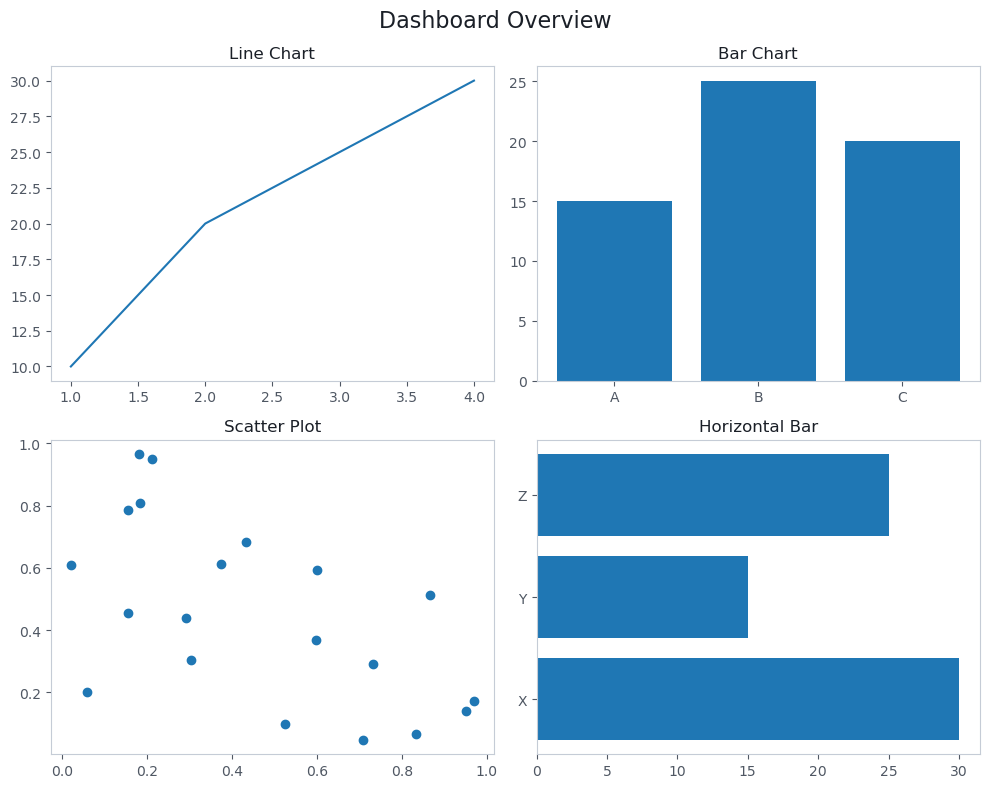
The key function is plt.subplots(nrows, ncols). It returns a figure and an array of axes objects. For a 2x2 grid, you get four axes you can plot on independently.

Creating a 2x2 subplot grid
import matplotlib
matplotlib.use('Agg')
import matplotlib.pyplot as plt
import numpy as np
# Create a 2x2 grid of subplots
fig, axes = plt.subplots(2, 2, figsize=(10, 8))
# Top-left: line chart
axes[0, 0].plot([1, 2, 3, 4], [10, 20, 25, 30])
axes[0, 0].set_title('Line Chart')
# Top-right: bar chart
axes[0, 1].bar(['A', 'B', 'C'], [15, 25, 20])
axes[0, 1].set_title('Bar Chart')
# Bottom-left: scatter plot
np.random.seed(42)
axes[1, 0].scatter(np.random.rand(20), np.random.rand(20))
axes[1, 0].set_title('Scatter Plot')
# Bottom-right: horizontal bar
axes[1, 1].barh(['X', 'Y', 'Z'], [30, 15, 25])
axes[1, 1].set_title('Horizontal Bar')
fig.suptitle('Dashboard Overview', fontsize=16)
fig.tight_layout()
print('Grid shape:', axes.shape)
print('Subplot titles:', [ax.get_title() for row in axes for ax in row])
print('Figure title:', fig.texts[0].get_text() if fig.texts else 'None')
Output
Grid shape: (2, 2)
Subplot titles: ['Line Chart', 'Bar Chart', 'Scatter Plot', 'Horizontal Bar']
Figure title: Dashboard Overview
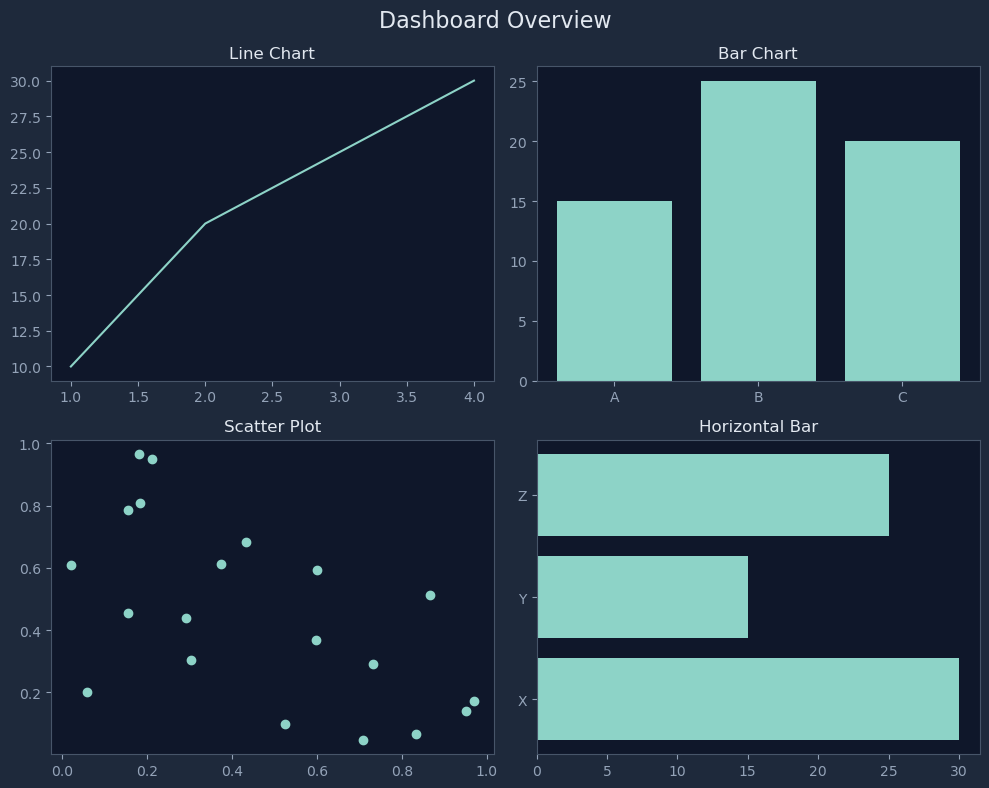
Chart drawn by: Creating a 2x2 subplot gridChart drawn by: Creating a 2x2 subplot grid

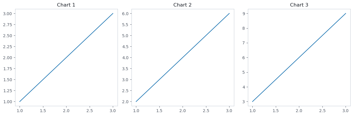
When you have a single row or column of subplots, the axes array is 1D instead of 2D. You can force it to always be 2D with squeeze=False, but for simple cases, just index directly.

Single row of subplots
import matplotlib
matplotlib.use('Agg')
import matplotlib.pyplot as plt
# Single row: axes is a 1D array
fig, axes = plt.subplots(1, 3, figsize=(12, 4))
for i, ax in enumerate(axes):
ax.plot([1, 2, 3], [i+1, (i+1)*2, (i+1)*3])
ax.set_title(f'Chart {i+1}')
fig.tight_layout()
print('Axes shape:', axes.shape)
print('Titles:', [ax.get_title() for ax in axes])
Output
Axes shape: (3,)
Titles: ['Chart 1', 'Chart 2', 'Chart 3']
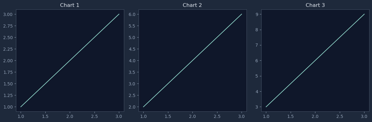
Chart drawn by: Single row of subplotsChart drawn by: Single row of subplots

How Do Twin Axes Show Two Different Scales?

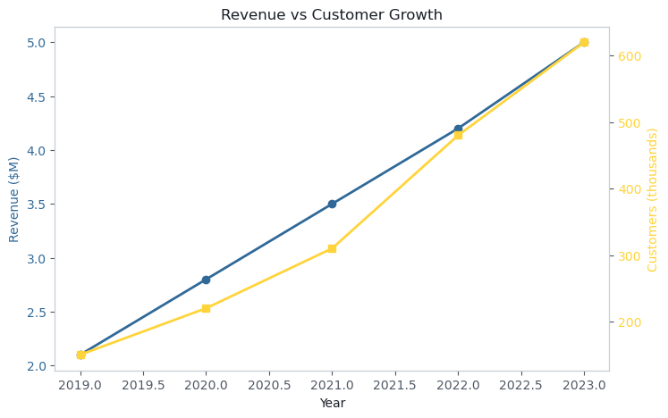
Sometimes you need to show two datasets that have completely different units. Imagine revenue (in millions of dollars) and customer count (in thousands) on the same chart. If you plot them on the same y-axis, the smaller numbers would be squashed flat.

Twin axes solve this by adding a second y-axis on the right side of the chart. Each dataset gets its own scale, but they share the same x-axis so you can see how they relate over time.

Dual y-axis chart
import matplotlib
matplotlib.use('Agg')
import matplotlib.pyplot as plt
years = [2019, 2020, 2021, 2022, 2023]
revenue = [2.1, 2.8, 3.5, 4.2, 5.0] # Millions
customers = [150, 220, 310, 480, 620] # Thousands
fig, ax1 = plt.subplots(figsize=(8, 5))
# Left y-axis: revenue
color1 = '#306998'
ax1.plot(years, revenue, color=color1, marker='o', linewidth=2, label='Revenue')
ax1.set_xlabel('Year')
ax1.set_ylabel('Revenue ($M)', color=color1)
ax1.tick_params(axis='y', labelcolor=color1)
# Right y-axis: customers (shares the same x-axis)
ax2 = ax1.twinx()
color2 = '#FFD43B'
ax2.plot(years, customers, color=color2, marker='s', linewidth=2, label='Customers')
ax2.set_ylabel('Customers (thousands)', color=color2)
ax2.tick_params(axis='y', labelcolor=color2)
ax1.set_title('Revenue vs Customer Growth')
print('Left y-axis label:', ax1.get_ylabel())
print('Right y-axis label:', ax2.get_ylabel())
print('Both share x-axis:', ax1.get_shared_x_axes().joined(ax1, ax2))
Output
Left y-axis label: Revenue ($M)
Right y-axis label: Customers (thousands)
Both share x-axis: True
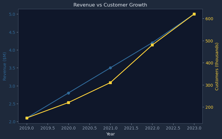
Chart drawn by: Dual y-axis chartChart drawn by: Dual y-axis chart

How Do You Annotate Key Data Points?

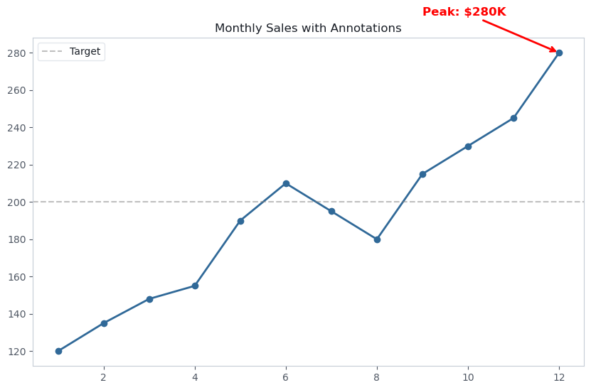
Annotations are like sticky notes on your chart. They point to specific data points and explain what's happening - a peak, a dip, a milestone. Good annotations turn a chart from "here's some data" into "here's what the data means."

Annotating data points
import matplotlib
matplotlib.use('Agg')
import matplotlib.pyplot as plt
months = list(range(1, 13))
sales = [120, 135, 148, 155, 190, 210, 195, 180, 215, 230, 245, 280]
fig, ax = plt.subplots(figsize=(10, 6))
ax.plot(months, sales, marker='o', color='#306998', linewidth=2)
# Find the peak and annotate it
peak_month = months[sales.index(max(sales))]
peak_value = max(sales)
ax.annotate(
f'Peak: ${peak_value}K',
xy=(peak_month, peak_value), # Point to annotate
xytext=(peak_month - 3, peak_value + 20), # Text position
fontsize=12,
fontweight='bold',
arrowprops=dict(arrowstyle='->', color='red', linewidth=2),
color='red'
)
# Add a horizontal reference line
ax.axhline(y=200, color='gray', linestyle='--', alpha=0.5, label='Target')
ax.set_title('Monthly Sales with Annotations')
ax.legend()
print('Peak month:', peak_month)
print('Peak value:', peak_value)
print('Number of annotations:', len(ax.texts))
print('Reference lines:', len([l for l in ax.lines if l.get_linestyle() == '--']))
Output
Peak month: 12
Peak value: 280
Number of annotations: 1
Reference lines: 1
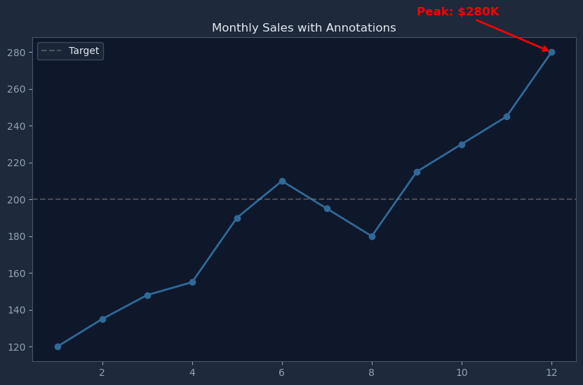
Chart drawn by: Annotating data pointsChart drawn by: Annotating data points

The annotate() function takes two key coordinates: xy is where the arrow points (the data point), and xytext is where the text label sits. The arrowprops dictionary controls the arrow style.

How Do Built-in Styles Transform Your Charts?

Matplotlib's default style is... functional but plain. The good news is that matplotlib ships with dozens of built-in styles that change the entire look of your charts with a single line of code.

Available matplotlib styles
import matplotlib
matplotlib.use('Agg')
import matplotlib.pyplot as plt
# List all available styles
styles = plt.style.available
print('Total styles available:', len(styles))
print('\nPopular styles:')
for s in sorted(styles):
if any(name in s for name in ['ggplot', 'seaborn', 'dark', 'fivethirtyeight', 'bmh']):
print(f' - {s}')
Output
Total styles available: 28

Popular styles:
 - bmh
 - dark_background
 - fivethirtyeight
 - ggplot
 - seaborn-v0_8
 - seaborn-v0_8-bright
 - seaborn-v0_8-colorblind
 - seaborn-v0_8-dark
 - seaborn-v0_8-dark-palette
 - seaborn-v0_8-darkgrid
 - seaborn-v0_8-deep
 - seaborn-v0_8-muted
 - seaborn-v0_8-notebook
 - seaborn-v0_8-paper
 - seaborn-v0_8-pastel
 - seaborn-v0_8-poster
 - seaborn-v0_8-talk
 - seaborn-v0_8-ticks
 - seaborn-v0_8-white
 - seaborn-v0_8-whitegrid
Applying a style
import matplotlib
matplotlib.use('Agg')
import matplotlib.pyplot as plt
# Apply a style
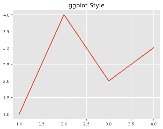
plt.style.use('ggplot')
fig, ax = plt.subplots()
ax.plot([1, 2, 3, 4], [1, 4, 2, 3], linewidth=2)
ax.set_title('ggplot Style')
# Check the background color to verify style is applied
face_color = ax.get_facecolor()
print('Style applied: ggplot')
print('Background color (RGBA):', tuple(round(c, 2) for c in face_color))
print('The ggplot style uses a light gray background with colored grid lines')
# Reset style for other examples
plt.style.use('default')
Output
Style applied: ggplot
Background color (RGBA): (0.9, 0.9, 0.9, 1.0)
The ggplot style uses a light gray background with colored grid lines
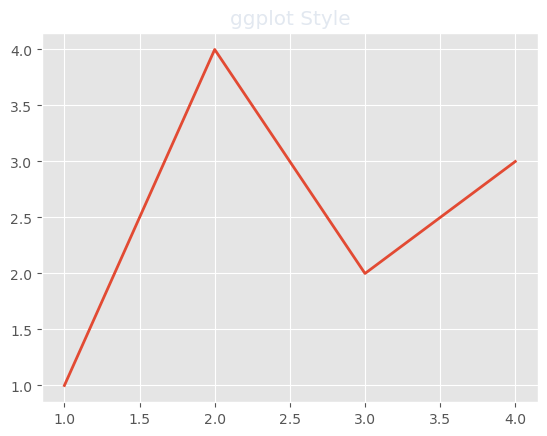
Chart drawn by: Applying a styleChart drawn by: Applying a style

What Are Colormaps and When Do You Use Them?

A colormap is a mapping from numbers to colors. Instead of manually picking colors for 50 data points, you give matplotlib a range of values and it automatically assigns colors from a gradient. This is essential for heatmaps, contour plots, and any visualization where color represents a third dimension of data.

Colormaps in scatter plots
import matplotlib
matplotlib.use('Agg')
import matplotlib.pyplot as plt
import numpy as np
# Colormap categories
print('Colormap categories:')
print(' Sequential: viridis, plasma, inferno, magma (low-to-high)')
print(' Diverging: coolwarm, RdBu, seismic (negative-zero-positive)')
print(' Qualitative: Set1, Set2, tab10 (distinct categories)')
print()
# Using a colormap with scatter
np.random.seed(42)
x = np.random.rand(50)
y = np.random.rand(50)
values = np.random.rand(50) * 100 # Color based on these values
fig, ax = plt.subplots()
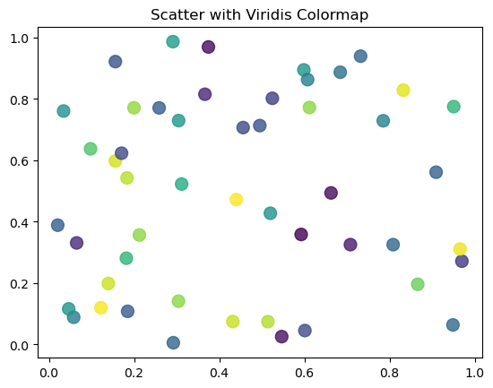
scatter = ax.scatter(x, y, c=values, cmap='viridis', s=100, alpha=0.8)
ax.set_title('Scatter with Viridis Colormap')
print('Points plotted:', len(x))
print('Value range: {:.1f} to {:.1f}'.format(values.min(), values.max()))
print('Colormap used: viridis')
print('Viridis goes from purple (low) through green to yellow (high)')
Output
Colormap categories:
  Sequential:  viridis, plasma, inferno, magma (low-to-high)
  Diverging:   coolwarm, RdBu, seismic (negative-zero-positive)
  Qualitative: Set1, Set2, tab10 (distinct categories)

Points plotted: 50
Value range: 0.7 to 97.2
Colormap used: viridis
Viridis goes from purple (low) through green to yellow (high)
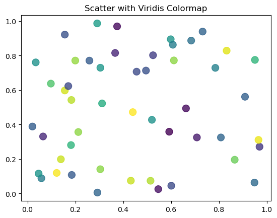
Chart drawn by: Colormaps in scatter plotsChart drawn by: Colormaps in scatter plots

Practice Exercises

Create a 1x3 Subplot Layout
Write Code

Create a figure with 1 row and 3 columns of subplots. Set the figure size to (12, 4). Set the titles of the three subplots to 'Sales', 'Profit', and 'Growth'. Call fig.tight_layout(), then print the shape of the axes array and the three titles.

import matplotlib
matplotlib.use('Agg')
import matplotlib.pyplot as plt
# Create 1x3 subplots with figsize (12, 4)
# Set titles for each subplot
# Call tight_layout
# Print axes shape and titles
Build a Dual-Axis Temperature and Humidity Chart
Write Code

Create a chart with twin y-axes. Plot temperature on the left axis and humidity on the right axis using ax1.twinx(). Set the left y-label to 'Temperature (C)' and the right y-label to 'Humidity (%)'. Print both y-axis labels.

import matplotlib
matplotlib.use('Agg')
import matplotlib.pyplot as plt
hours = list(range(0, 24, 3)) # 0, 3, 6, ..., 21
temperature = [18, 16, 15, 20, 25, 28, 26, 22]
humidity = [80, 85, 88, 70, 55, 45, 50, 65]
# Create figure and primary axis
# Plot temperature on left axis
# Create twin axis and plot humidity
# Set labels and print them
Annotate the Maximum Value
Write Code

Given the prices list, find the index and value of the maximum price. Plot the data, then use ax.annotate() to label the peak point with the text 'Peak: $MAX' (where MAX is the actual max value). Also add a horizontal dashed line at the average price using ax.axhline(). Print the max value and the average (rounded to 1 decimal).

import matplotlib
matplotlib.use('Agg')
import matplotlib.pyplot as plt
days = list(range(1, 11))
prices = [42, 45, 43, 48, 52, 49, 55, 53, 58, 54]
fig, ax = plt.subplots()
ax.plot(days, prices, marker='o')
# Find max value and its index
# Annotate the peak
# Add average reference line
# Print max and average
Predict the Subplot Configuration
Predict Output

What will this code print? Think carefully about the subplot grid shape and the tight_layout call.

import matplotlib
matplotlib.use('Agg')
import matplotlib.pyplot as plt
fig, axes = plt.subplots(2, 3, figsize=(15, 10))
for i in range(2):
for j in range(3):
axes[i, j].set_title(f'Plot {i*3 + j + 1}')
print(axes.shape)
print(axes[1, 2].get_title())
Create a Color-Coded Scatter Plot
Write Code

Create a scatter plot where point color represents a third variable. Use numpy to generate 30 random x, y, and scores values (seed 42). Use ax.scatter() with c=scores, cmap='plasma', and s=80. Print the number of points and the colormap name from the scatter collection.

import matplotlib
matplotlib.use('Agg')
import matplotlib.pyplot as plt
import numpy as np
np.random.seed(42)
x = np.random.rand(30)
y = np.random.rand(30)
scores = np.random.randint(0, 100, 30)
# Create scatter plot with colormap
# Print number of points and colormap name

Harder problems

More problems on this topic: Working with data

Related Tutorials

Was this tutorial helpful?